Welcome to our training for our Learner Support facilitators!! Your friendly ITEs will be guiding you through your workshop topics. Have some fun!

Bring what you do! Your class lists, reading logs, some lesson material for next term- let's see how you can make it easier for yourself!

Training Menu Day 3

Time	Session	Description	Skills and tools
Day 3 9:00–9:30	Icebreaker	Jaribaaaaa	Lots of jaribaaness
Day 3 9:30-10:00	Design a dream intervention for your learners	Discuss what your ideal reading room could be like.	4 C's
Day 3 10:00-10:45	Dream budget	You won R10000!!! Create a dream Budget for your intervention	Excel, AI,
Day 3 10:45-11:00	Tea break	Stir it up!	Slurp slurp
Day 3 11:00- 12:15	Dream budget	Dream budget continues	Excel
Day 3 12:15-13:00	Lunch	Njammie njammie	Gobbling
Day 3 13:00-14:00	Sorting stuff	Learn how to filter and sort	Excel Google sheets
Day 3 14:00-15:00	Happy sheet	Capturing data using forms and sheets	Google/MS forms Google/Excel sheets

Activity 1: Design your Dream Reading Room

This is a team activity. Let's dream! If we had an unlimited budget, what would we do, create or buy, to make the most amazing environment for our little readers? Spend some time discussing in your groups what you would like.

Ideas:

Check our our Wakelet for some reading room ideas and stuff!
Make a list of things that you really, really really would like and how much they cost.
Ask Chatgpt to help your team with ideas. What prompt could you give it?

Activity 2: You won R10 000. Create your dream reading room

Let's see how far R10 000 can get you to realise your dream reading room. Creating a budget is a great way to practice your Spreadsheet skills while letting your dreams run wild!

In this exercise, you will apply basic formatting, adjust column widths, and use formulas to calculate the cheapest items using the min function!

Instructions:

Step 1: Create your budget spreadsheet and title

Open Excel /Google sheets and create a new worksheet.
Save it as Budget.yourname.xlsx
In Cell A1, type: Reading Room budget
- Make the Font: Size 20, Bold
- Fill color: Purple or any colour of your choice
- Merge & Center across columns A to H (Highlight and click on Merge in the ribbon)

Step 2: Enter Column Headers in Row 2

Format Row 2 (Headers):
- Font: Size 14, Bold
- Change Cell Fill color for cells 2A to 2H to Yellow
- Change column size to fit or wrap the headings to fit. (drag the handles at the top between the letters).

Step 3: Add Your Budget Items Rows 3 to ...

Make the font size from cells A3 to H14 Size 14 (click and drag to highlight and then click on font size 14.
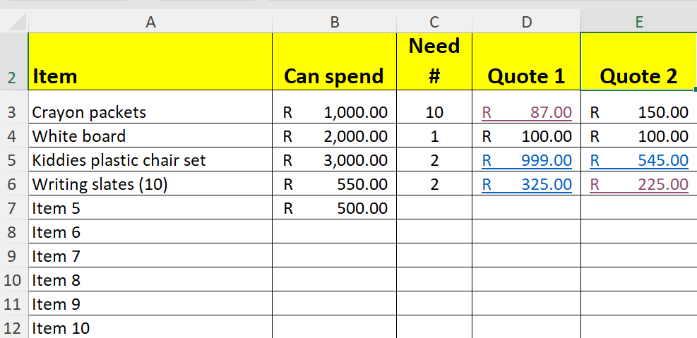
Under the Item column header A, list all your dream items that you would like to buy. Remember you only have R10 000! It won't show the R, we will add that later.
- Bold the items
Column B (Can spend): Put in how much you would like to spend next to each item
In Column C, put in the number of items you will need
Research some online quotes for your items (e.g. Takelot, Temu, Makro, Parrot, Mambos) and find the best buy. Have some fun with it!
- Google the items. It will always give you a list with pictures of the sponsored items.
In Columns D and E add the amounts that each item will cost from 2 different vendors
(e.g. Crayons cost R87 at Takelot but R150 at Parrot)

Step 4 - Apply Formulas Did we over spend?

One row below your last Item entry, type in Totals (e.g. A13)
- Bold the whole Row from A to H so that you can see where you are going tom put your forumals in.
Underneath the Can Spend column B enter the following formula by clicking on where you want the formula to be (eg. in cell B13)
Now type =sum(B3:B12)
A quick way to do this B3:B12 is to click on B3 and drag to B12.
Don't forget to complete your formula by putting in the end bracket and hitting enter!! Voila!
Copy the formula that you created in cell B13 to all the adjacent cells (C13 to G13) by dragging the handle in the bottom right corner of the cell.

In Cell F3 add the following formula =min(D3:E3)
Copy the formula (Click and drag the bottom right corner of the cell to the bottom of your list in column F. You now have all the cheapest prices in column F and what it will all cost in total in the last row!
In cell G3 do the following formula: =F3*C3 The * in computer language means multiply. So we are multiplying the cheapest amount by the number of items to get the total cost in cell G3.
Copy the formula in cell G3 (Click and drag the bottom right corner of the cell to the bottom of your list in column G. You now have all the cheapest prices in column F and what it will all cost in total in the last row!
Complete the last column by entering your chosen vendor for each item in column H.

In the row underneath the Totals cell (A13--> in A14) type Budgeted amount and in B14 put in your 10 000.
In cell E14 type in Actual amount and in the cell next to it =G13 (or click on the cell above it.

Step 5 - Making your table look pretty- Formatting

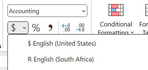
Highlight B3 to G13 (last cell calculation) and change the numbers into Rands:
Highlight --> click B3 drag to G13 --> under accounting, click on $ dropdown and on R

Activity 3: Sorting your stuff (data sort and filters)

Download and open the spreadsheet and save under your own name sort.yourname.xlsx

Open sorting spreadsheet
Excel

Open sorting spreadsheet
Google sheets

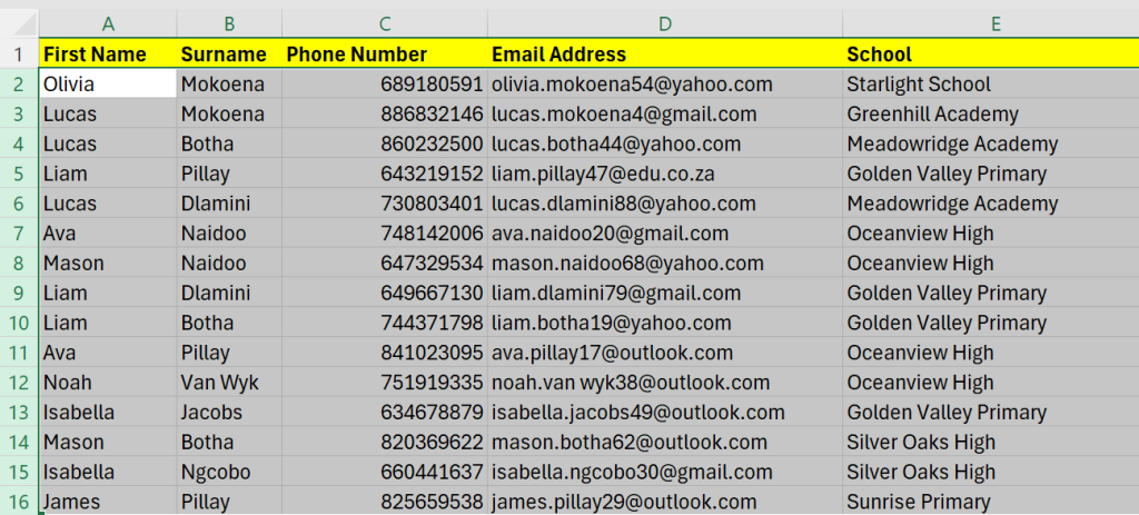
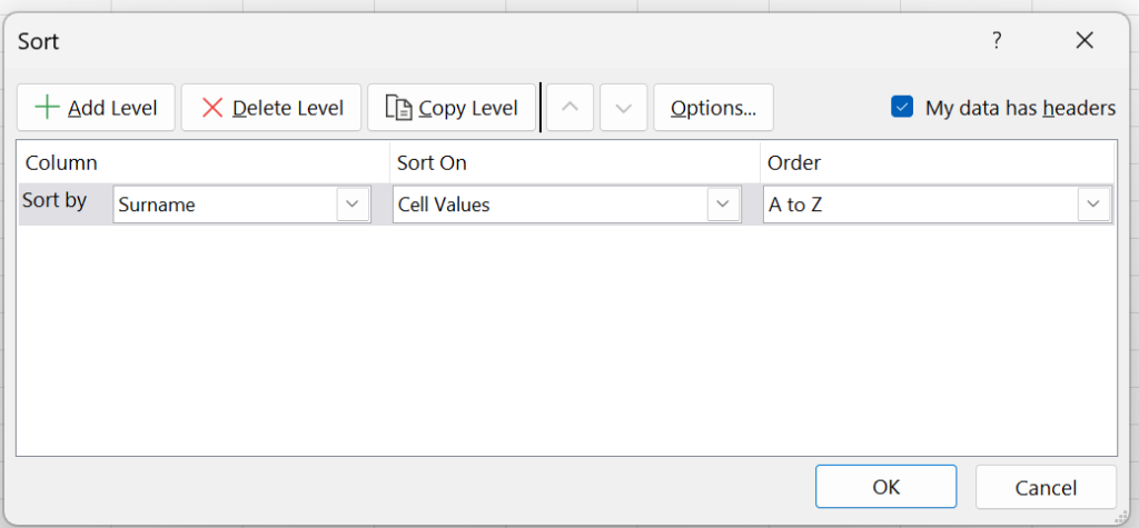
Sort the name list into alphabetical surname order (from A-Z)
- Highlight the rows that you want to sort (click on the row number hold down and drag to the number where you want to stop)
- Choose Sort by Surname --> cell values --> A to Z
- Voila!

Now try sorting for Schools

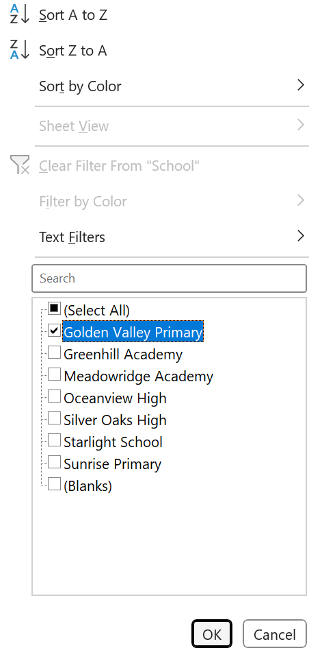
Sorting using filters

Select the whole sheet--> click on the top left hand space above the sheet (between the row and column headings

Click on the Filter command in the ribbon
You will now see little dropdown arrows on each heading

You can now filter for what you want
- Filter by school Golden Valley Primary (how many teachers?)
- Filter by surname.
To remove the filter just clear it or click on the filter command button to switch it off.

Can you do all of this now?

Thank you for getting a basic understanding of how valuable Excel can be for you. If you want to learn more about Excel, we recommend trying the beginner's certification for Excel, which you can add to your CV. See the next activity.

You have to be able to:

Launch MS Excel
Create a new workbook.
Type text or numbers into a cell.
Basic formula use (add, subtract, divide and
multiply)
Can resize columns and rows.
Able to zoom in and out
Able to select a cell, copy and paste or move it.
Able to select a range of cells, copy and paste or move them.
Open a recently used document.
Print a document - fit entire worksheet on one page.
Print a worksheet - fit all columns on one page.
Save the workbook.
Close MS Excel.
All basic skills, including:
- Place borders around a cell or range of cells.
- Shade a cell or a range of cells.
- Can use the Autofill feature.
- Change font type, size and colour.
Can use the following functions:
- SUM, AVERAGE, MAX, MIN, COUNT
Can use the apostrophe to prevent cells doing automatic date/time/dropped zero.
Print/Export to PDF.
Uses cell references instead of typing in values.
Can sort a column, or range, numerically or alphabetically.
Knows at least three keyboard shortcuts for MS Excel.
Can access Help within Excel.
Understands the differences between the various number, date, and currency formats in the ‘Number’ group on the ribbon.

Sign Happy sheet

Excel Beginner Certification

Register for an account on the GFCGlobal platform
Complete the Excel GCFGlobal course. Make sure that you make notes as you go along. Watch the videos and complete the tasks within the course.
Complete the Excel assessment and download the certificate.