Welcome to our training for our Vocational Focus learners!! Your friendly ITEs will be guiding you through your workshop topics. Have some fun!

The criteria for the Excel Badge are as follows:

Please make sure that you can do ALL of the items below. If you can't do it, please ask your friendly ITE for support. You have to be able to:

• Launch MS Excel
• Create a new workbook.
• Type text or numbers into a cell.
• Basic formula use (add, subtract, divide and
• multiply)
• Can resize columns and rows.
• Able to zoom in and out
• Able to select a cell, copy and paste or move it.
• Able to select a range of cells, copy and paste or move them.
• Open a recently used document.
• Print a document - fit entire worksheet on one page.
• Print a worksheet - fit all columns on one page.
• Save the workbook.
• Close MS Excel.
• All basic skills, including:
  • Place borders around a cell or range of cells.
  • Shade a cell or a range of cells.
  • Can use the Autofill feature.
  • Change font type, size and colour.
• Can use the following functions:
  • SUM, AVERAGE, MAX, MIN, COUNT
• Can use the apostrophe to prevent cells doing automatic date/time/dropped zero.
• Print/Export to PDF.
• Uses cell references instead of typing in values.
• Can sort a column, or range, numerically or alphabetically.
• Knows at least three keyboard shortcuts for MS Excel.
• Can access Help within Excel.
• Understands the differences between the various number, date and currency formats in the ‘Number’ group on the ribbon.

Activity 1: Achie Breakie Heart

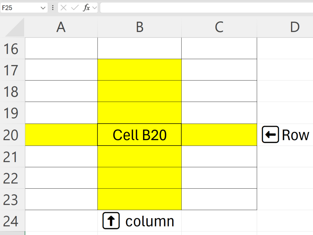
In this exercise, you will construct a robot heart and find your way around an Excel spreadsheet. So get your groove on with rows and columns! The facilitator will yell out the spreadsheet cell locations (what is a row, column and cell?) for you to colour in (red- how? )

Instructions:

• Open up an Excel workbook (How?)
• Save the spreadsheet under your name (File--> Save as--> yournamegr11.xlsx) The part behind the file name tells us that it is an Excel spreadsheet (.xlsx)
• Are we ready? Let's go!
• Highlight columns B all the way to K and drag the column line on top so that the cells between B and K are all square.
• Colour in all the following cells (red) to the tune of achie breakie heart!!
  • F5, H8, G4, G6, C6, C7, E5, E9, F6, H7, F4, G5, D5, E8, I6, E6, E4, H4, C5, D6, I5, G7, H6, G3, D7, E7, H5, E3, I7, F7, G6, F9, G9, F8, F10, G5, D4, G8
  • Break the heart with a black crack through it (colour some of the blocks black)
• Draw a nice thick frame around the heart (Highlight the heart--> Click and pick borders in the ribbon
• Merge B1-K1 and insert the following phrase: My name is ..... and I have an achie breakie heart
• As it does not fit, wrap the text and drag rows until you can see all your typing.
• Your Facilitator will create a TikTok of you and your robot heart (play the part!!

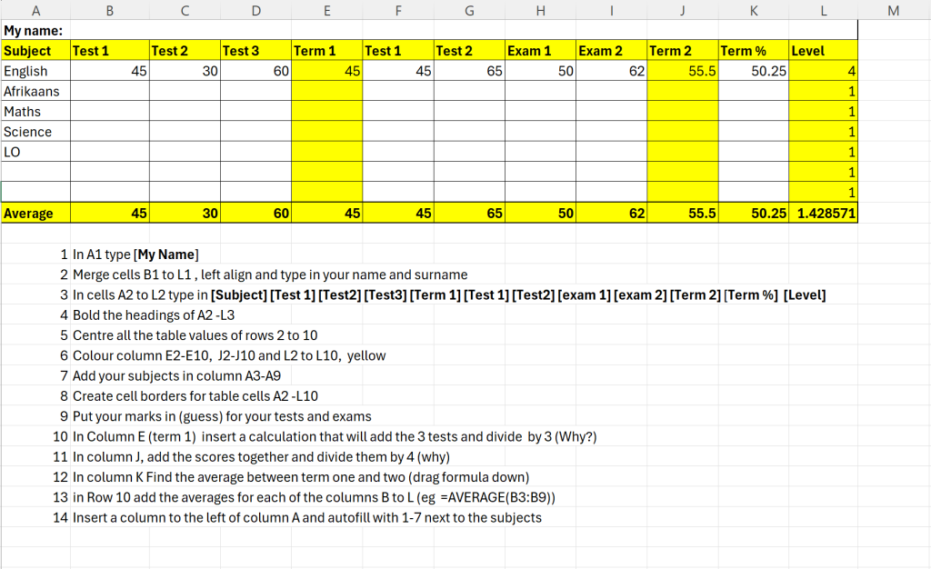
Activity 2: How do the teachers work out our marks?

Activity 4: GCF Excel Wrap-Up Challenge

1. Complete the excel GCFGlobal course.
2. Save it in your POE folder with the file name excelbadge_YournameYoursurname.pdf e.g. excelbadgeMaggieVerster.pdf. (Upload your certificate to your school (teacher) folder (ask your ITE for the POE link).
3. Create an email and attach your certificate to the email.
4. Make sure that you use the relevant formal email etiquette.
5. Send the email to:
   • Grade 12s: gr12poe@klearning.co.za and cc Nonqaba (nonqabac@kilt.org.za)

Step 3: Enter Data

1. Font: Size 18
2. Under the "Item" column, enter the following expenses for the Matric Dance:
   
   • Dress/Suit
     
   • Shoes
     
   • Accessories
     
   • Transport
     
3. For each item, enter price estimates from three different stores.
4. Enter the budgeted amount for each item in the "Budgeted Price" column.
5. Choose the best price for each item and enter it in the "Chosen Price" column.

Step 4: Apply Formulas

Calculate the Difference:
Formula for Difference (H3):
=MIN(F3-E3)

• Copy down for all rows.
  
• If the result is positive → You saved money.
  
• If negative → You overspent.
  

Calculate the Average Price:

• Formula for Average Price (I3):
  
  =AVERAGE(B3:D3)

Calculate the Total for Each Column (Row 8):

Total Chosen Price (E8):
=SUM(E3:E7)

Total Budgeted Price (F8):
=SUM(F3:F7)

Total Difference (G8):
=SUM(G3:G7)

Total Average Price (H8):
=AVERAGE(H3:H7)

Step 5: Apply Conditional Formatting to the "Difference" Column

Step 6: Borders

• Apply borders around all cells (A2:H9) except for the title (A1)

Step 7: Set Currency Formatting

• Select columns B to H (all price-related columns).
• Click "Home" → "Number Format" → "Currency (R)

Step 8: Add the Stores You Visited

• Scroll down to Cell A11 on your Excel sheet — just below your budget table.
• Create a mini table starting in Cell A11 to record the names of the stores you used to get prices for the following items:

A11: Item

B11: Store 1 Name

C11: Store 2 Name

D11: Store 3 Name

• In the next rows, enter the item names and the store names where you found the prices. It should look something like this:
• Add borders to your mini store table to match the main budget sheet formatting.

Step 9: Save and Review

• Save the file as Matric Dance Budget_YournameYoursurname.xlsx.
• Review the data, ensuring that formulas and conditional formatting work correctly.
  

Step 10: Email Exercise

1. Save it in your POE folder with the file name Matric Dance Budget_YournameYoursurname.xlsx e.g. Matric Dance Budget_MaggieVerster.xlsx.
2. Create an email. Make sure that you use the relevant formal email etiquette.
3.  Attach your Matric Dance Budget Sheet.
4. Send the email to:
5. Grade 12s: gr12poe@klearning.co.za and cc Nonqaba (nonqabac@kilt.org.za)